1 + 1[1] 2Please review the following sections for instructions on installation steps:
While it makes sense to use Quarto going forward, there are still a lot of resources written for and in R Markdown. For this reason we provide the R Markdown equivalents for this section in Appendix.
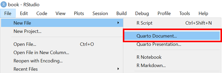
In RStudio, you can create a new Quarto document by selecting File > New File > Quarto Document…
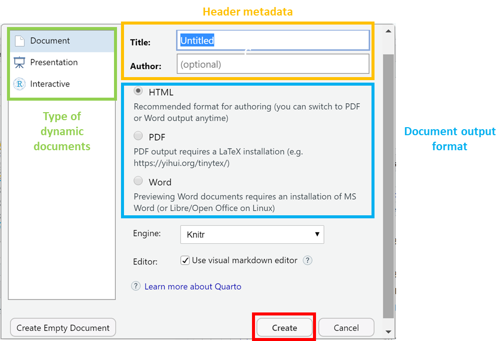
When you create a new Quarto document, RStudio tries to be helpful by allowing you to select a template which explains the different section of an R Markdown script. R Studio will enable you select options to pick from to generate a template Quarto document to start from.
The title and the author names are not important. If the output document type you want is not one of these, do not worry - you can just pick any one and change it later.
Let us select HTML to create an html document.
Click on create to open up a new Quarto (.Qmd) document.
The RStudio Visual Editor is quite new and has features that improve your writing experience. Working in the Visual Editor feels a bit like working in a Google Doc.
Here’s an example showing the same file in the original Source Editor with content in markdown format and in the Visual Editor with content that looks more like it will appear in a live site. You can switch freely between these modes.
An R Markdown document can be edited in RStudio.
There are three basic components to a Quarto document, similar to the components of a R Markdown document:
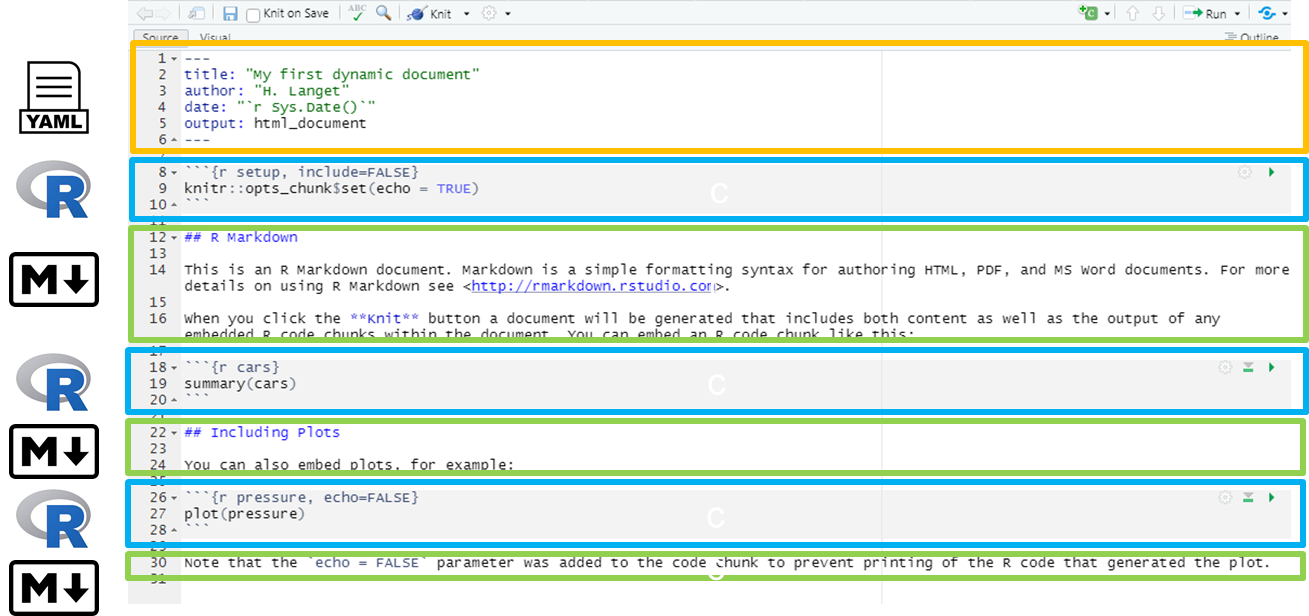
The very top of the document consists of a (YAML) header surrounded by — lines. Here you may want to edit the title of your document. The other settings in the header define the default document type produced (Microsoft Word) when the RMarkdown is “knit”. the information intended to produce an html output.
In WHITE background areas, any text will appear as regular text in the final report. Can have formatting such as headings, italics, bold, numbers, and bullets. See the second page of this RMarkdown cheatsheet for more detail. Can display parameters derived from your data via in-line code (such as epi week of the outbreak peak, as in the example above).
In gray background “code chunks”, RMarkdown is running R commands. These commands perform data processing and cleaning steps, or could produce visual outputs in the document.
When you click the Render button a document will be generated that includes both content and the output of embedded code.
 ## Code options
You can embed code like this:
1 + 1[1] 2You can add options to executable code like this
[1] 4The echo: false option disables the printing of code (only output is displayed).
As the number of programming languages used for scientific discourse is very broad, Quarto was developed to be multilingual, beginning with R, Python, Javascript, and Julia. building on the RStudio (R) and Jupyter (Python, Julia) ecosystems which are very popular. Stata is not a language supported by Quarto.
To write and execute code in Quarto, you will use code chunks.
Here are some tips for creating code chunks in RStudio
Ctrl + Alt + IIn this section, we will see how to use and mix R, Stata and Python within Quarto so that you can make the most out of it.
A data frame is a two-dimensional array-like structure that contains rows and columns.
To store the content of the iris dataset into a data frame named df, you can use = (equal) but good practice recommend using <- (back arrow) to indicate the direction of your allocation.
```{r}
df <- iris
```
How to display data
```{r}
#| df-print: kable
library(dplyr)
```
Attache Paket: 'dplyr'Die folgenden Objekte sind maskiert von 'package:stats':
filter, lagDie folgenden Objekte sind maskiert von 'package:base':
intersect, setdiff, setequal, union```{r}
#| df-print: kable
knitr::kable(head(df, 10))
```| Sepal.Length | Sepal.Width | Petal.Length | Petal.Width | Species |
|---|---|---|---|---|
| 5.1 | 3.5 | 1.4 | 0.2 | setosa |
| 4.9 | 3.0 | 1.4 | 0.2 | setosa |
| 4.7 | 3.2 | 1.3 | 0.2 | setosa |
| 4.6 | 3.1 | 1.5 | 0.2 | setosa |
| 5.0 | 3.6 | 1.4 | 0.2 | setosa |
| 5.4 | 3.9 | 1.7 | 0.4 | setosa |
| 4.6 | 3.4 | 1.4 | 0.3 | setosa |
| 5.0 | 3.4 | 1.5 | 0.2 | setosa |
| 4.4 | 2.9 | 1.4 | 0.2 | setosa |
| 4.9 | 3.1 | 1.5 | 0.1 | setosa |
The pipe operator
```{r}
#| df-print: kable
library(dplyr)
df %>%
  head(10) %>%
  knitr::kable()
```| Sepal.Length | Sepal.Width | Petal.Length | Petal.Width | Species |
|---|---|---|---|---|
| 5.1 | 3.5 | 1.4 | 0.2 | setosa |
| 4.9 | 3.0 | 1.4 | 0.2 | setosa |
| 4.7 | 3.2 | 1.3 | 0.2 | setosa |
| 4.6 | 3.1 | 1.5 | 0.2 | setosa |
| 5.0 | 3.6 | 1.4 | 0.2 | setosa |
| 5.4 | 3.9 | 1.7 | 0.4 | setosa |
| 4.6 | 3.4 | 1.4 | 0.3 | setosa |
| 5.0 | 3.4 | 1.5 | 0.2 | setosa |
| 4.4 | 2.9 | 1.4 | 0.2 | setosa |
| 4.9 | 3.1 | 1.5 | 0.1 | setosa |
You can cross-reference your table Table 12.1
```{r}
#| label: tbl-iris
#| tbl-cap: Iris data set
#| df-print: kable
df %>%
  knitr::kable()
```| Sepal.Length | Sepal.Width | Petal.Length | Petal.Width | Species |
|---|---|---|---|---|
| 5.1 | 3.5 | 1.4 | 0.2 | setosa |
| 4.9 | 3.0 | 1.4 | 0.2 | setosa |
| 4.7 | 3.2 | 1.3 | 0.2 | setosa |
| 4.6 | 3.1 | 1.5 | 0.2 | setosa |
| 5.0 | 3.6 | 1.4 | 0.2 | setosa |
| 5.4 | 3.9 | 1.7 | 0.4 | setosa |
| 4.6 | 3.4 | 1.4 | 0.3 | setosa |
| 5.0 | 3.4 | 1.5 | 0.2 | setosa |
| 4.4 | 2.9 | 1.4 | 0.2 | setosa |
| 4.9 | 3.1 | 1.5 | 0.1 | setosa |
| 5.4 | 3.7 | 1.5 | 0.2 | setosa |
| 4.8 | 3.4 | 1.6 | 0.2 | setosa |
| 4.8 | 3.0 | 1.4 | 0.1 | setosa |
| 4.3 | 3.0 | 1.1 | 0.1 | setosa |
| 5.8 | 4.0 | 1.2 | 0.2 | setosa |
| 5.7 | 4.4 | 1.5 | 0.4 | setosa |
| 5.4 | 3.9 | 1.3 | 0.4 | setosa |
| 5.1 | 3.5 | 1.4 | 0.3 | setosa |
| 5.7 | 3.8 | 1.7 | 0.3 | setosa |
| 5.1 | 3.8 | 1.5 | 0.3 | setosa |
| 5.4 | 3.4 | 1.7 | 0.2 | setosa |
| 5.1 | 3.7 | 1.5 | 0.4 | setosa |
| 4.6 | 3.6 | 1.0 | 0.2 | setosa |
| 5.1 | 3.3 | 1.7 | 0.5 | setosa |
| 4.8 | 3.4 | 1.9 | 0.2 | setosa |
| 5.0 | 3.0 | 1.6 | 0.2 | setosa |
| 5.0 | 3.4 | 1.6 | 0.4 | setosa |
| 5.2 | 3.5 | 1.5 | 0.2 | setosa |
| 5.2 | 3.4 | 1.4 | 0.2 | setosa |
| 4.7 | 3.2 | 1.6 | 0.2 | setosa |
| 4.8 | 3.1 | 1.6 | 0.2 | setosa |
| 5.4 | 3.4 | 1.5 | 0.4 | setosa |
| 5.2 | 4.1 | 1.5 | 0.1 | setosa |
| 5.5 | 4.2 | 1.4 | 0.2 | setosa |
| 4.9 | 3.1 | 1.5 | 0.2 | setosa |
| 5.0 | 3.2 | 1.2 | 0.2 | setosa |
| 5.5 | 3.5 | 1.3 | 0.2 | setosa |
| 4.9 | 3.6 | 1.4 | 0.1 | setosa |
| 4.4 | 3.0 | 1.3 | 0.2 | setosa |
| 5.1 | 3.4 | 1.5 | 0.2 | setosa |
| 5.0 | 3.5 | 1.3 | 0.3 | setosa |
| 4.5 | 2.3 | 1.3 | 0.3 | setosa |
| 4.4 | 3.2 | 1.3 | 0.2 | setosa |
| 5.0 | 3.5 | 1.6 | 0.6 | setosa |
| 5.1 | 3.8 | 1.9 | 0.4 | setosa |
| 4.8 | 3.0 | 1.4 | 0.3 | setosa |
| 5.1 | 3.8 | 1.6 | 0.2 | setosa |
| 4.6 | 3.2 | 1.4 | 0.2 | setosa |
| 5.3 | 3.7 | 1.5 | 0.2 | setosa |
| 5.0 | 3.3 | 1.4 | 0.2 | setosa |
| 7.0 | 3.2 | 4.7 | 1.4 | versicolor |
| 6.4 | 3.2 | 4.5 | 1.5 | versicolor |
| 6.9 | 3.1 | 4.9 | 1.5 | versicolor |
| 5.5 | 2.3 | 4.0 | 1.3 | versicolor |
| 6.5 | 2.8 | 4.6 | 1.5 | versicolor |
| 5.7 | 2.8 | 4.5 | 1.3 | versicolor |
| 6.3 | 3.3 | 4.7 | 1.6 | versicolor |
| 4.9 | 2.4 | 3.3 | 1.0 | versicolor |
| 6.6 | 2.9 | 4.6 | 1.3 | versicolor |
| 5.2 | 2.7 | 3.9 | 1.4 | versicolor |
| 5.0 | 2.0 | 3.5 | 1.0 | versicolor |
| 5.9 | 3.0 | 4.2 | 1.5 | versicolor |
| 6.0 | 2.2 | 4.0 | 1.0 | versicolor |
| 6.1 | 2.9 | 4.7 | 1.4 | versicolor |
| 5.6 | 2.9 | 3.6 | 1.3 | versicolor |
| 6.7 | 3.1 | 4.4 | 1.4 | versicolor |
| 5.6 | 3.0 | 4.5 | 1.5 | versicolor |
| 5.8 | 2.7 | 4.1 | 1.0 | versicolor |
| 6.2 | 2.2 | 4.5 | 1.5 | versicolor |
| 5.6 | 2.5 | 3.9 | 1.1 | versicolor |
| 5.9 | 3.2 | 4.8 | 1.8 | versicolor |
| 6.1 | 2.8 | 4.0 | 1.3 | versicolor |
| 6.3 | 2.5 | 4.9 | 1.5 | versicolor |
| 6.1 | 2.8 | 4.7 | 1.2 | versicolor |
| 6.4 | 2.9 | 4.3 | 1.3 | versicolor |
| 6.6 | 3.0 | 4.4 | 1.4 | versicolor |
| 6.8 | 2.8 | 4.8 | 1.4 | versicolor |
| 6.7 | 3.0 | 5.0 | 1.7 | versicolor |
| 6.0 | 2.9 | 4.5 | 1.5 | versicolor |
| 5.7 | 2.6 | 3.5 | 1.0 | versicolor |
| 5.5 | 2.4 | 3.8 | 1.1 | versicolor |
| 5.5 | 2.4 | 3.7 | 1.0 | versicolor |
| 5.8 | 2.7 | 3.9 | 1.2 | versicolor |
| 6.0 | 2.7 | 5.1 | 1.6 | versicolor |
| 5.4 | 3.0 | 4.5 | 1.5 | versicolor |
| 6.0 | 3.4 | 4.5 | 1.6 | versicolor |
| 6.7 | 3.1 | 4.7 | 1.5 | versicolor |
| 6.3 | 2.3 | 4.4 | 1.3 | versicolor |
| 5.6 | 3.0 | 4.1 | 1.3 | versicolor |
| 5.5 | 2.5 | 4.0 | 1.3 | versicolor |
| 5.5 | 2.6 | 4.4 | 1.2 | versicolor |
| 6.1 | 3.0 | 4.6 | 1.4 | versicolor |
| 5.8 | 2.6 | 4.0 | 1.2 | versicolor |
| 5.0 | 2.3 | 3.3 | 1.0 | versicolor |
| 5.6 | 2.7 | 4.2 | 1.3 | versicolor |
| 5.7 | 3.0 | 4.2 | 1.2 | versicolor |
| 5.7 | 2.9 | 4.2 | 1.3 | versicolor |
| 6.2 | 2.9 | 4.3 | 1.3 | versicolor |
| 5.1 | 2.5 | 3.0 | 1.1 | versicolor |
| 5.7 | 2.8 | 4.1 | 1.3 | versicolor |
| 6.3 | 3.3 | 6.0 | 2.5 | virginica |
| 5.8 | 2.7 | 5.1 | 1.9 | virginica |
| 7.1 | 3.0 | 5.9 | 2.1 | virginica |
| 6.3 | 2.9 | 5.6 | 1.8 | virginica |
| 6.5 | 3.0 | 5.8 | 2.2 | virginica |
| 7.6 | 3.0 | 6.6 | 2.1 | virginica |
| 4.9 | 2.5 | 4.5 | 1.7 | virginica |
| 7.3 | 2.9 | 6.3 | 1.8 | virginica |
| 6.7 | 2.5 | 5.8 | 1.8 | virginica |
| 7.2 | 3.6 | 6.1 | 2.5 | virginica |
| 6.5 | 3.2 | 5.1 | 2.0 | virginica |
| 6.4 | 2.7 | 5.3 | 1.9 | virginica |
| 6.8 | 3.0 | 5.5 | 2.1 | virginica |
| 5.7 | 2.5 | 5.0 | 2.0 | virginica |
| 5.8 | 2.8 | 5.1 | 2.4 | virginica |
| 6.4 | 3.2 | 5.3 | 2.3 | virginica |
| 6.5 | 3.0 | 5.5 | 1.8 | virginica |
| 7.7 | 3.8 | 6.7 | 2.2 | virginica |
| 7.7 | 2.6 | 6.9 | 2.3 | virginica |
| 6.0 | 2.2 | 5.0 | 1.5 | virginica |
| 6.9 | 3.2 | 5.7 | 2.3 | virginica |
| 5.6 | 2.8 | 4.9 | 2.0 | virginica |
| 7.7 | 2.8 | 6.7 | 2.0 | virginica |
| 6.3 | 2.7 | 4.9 | 1.8 | virginica |
| 6.7 | 3.3 | 5.7 | 2.1 | virginica |
| 7.2 | 3.2 | 6.0 | 1.8 | virginica |
| 6.2 | 2.8 | 4.8 | 1.8 | virginica |
| 6.1 | 3.0 | 4.9 | 1.8 | virginica |
| 6.4 | 2.8 | 5.6 | 2.1 | virginica |
| 7.2 | 3.0 | 5.8 | 1.6 | virginica |
| 7.4 | 2.8 | 6.1 | 1.9 | virginica |
| 7.9 | 3.8 | 6.4 | 2.0 | virginica |
| 6.4 | 2.8 | 5.6 | 2.2 | virginica |
| 6.3 | 2.8 | 5.1 | 1.5 | virginica |
| 6.1 | 2.6 | 5.6 | 1.4 | virginica |
| 7.7 | 3.0 | 6.1 | 2.3 | virginica |
| 6.3 | 3.4 | 5.6 | 2.4 | virginica |
| 6.4 | 3.1 | 5.5 | 1.8 | virginica |
| 6.0 | 3.0 | 4.8 | 1.8 | virginica |
| 6.9 | 3.1 | 5.4 | 2.1 | virginica |
| 6.7 | 3.1 | 5.6 | 2.4 | virginica |
| 6.9 | 3.1 | 5.1 | 2.3 | virginica |
| 5.8 | 2.7 | 5.1 | 1.9 | virginica |
| 6.8 | 3.2 | 5.9 | 2.3 | virginica |
| 6.7 | 3.3 | 5.7 | 2.5 | virginica |
| 6.7 | 3.0 | 5.2 | 2.3 | virginica |
| 6.3 | 2.5 | 5.0 | 1.9 | virginica |
| 6.5 | 3.0 | 5.2 | 2.0 | virginica |
| 6.2 | 3.4 | 5.4 | 2.3 | virginica |
| 5.9 | 3.0 | 5.1 | 1.8 | virginica |