```{r}
# Write your code here
```5 :blue_book: Manipulate data
5.1 Introduction
Important
Remember that with Quarto you can store multiple data sets in memory (stored in different data frames df1, df2, df3, etc) and work in parallel on all these data sets.
5.2 Import data
Import dataset1.xlsx using Stata and store it in df1
```{r}
df1 <- openxlsx::read.xlsx("./data/dataset1a.xlsx")
```
5.3 Piping
Package dplyr
Pipes are a powerful tool for clearly expressing a sequence of multiple operations. So far, you’ve been using them without knowing how they work, or what the alternatives are. Now, in this chapter, it’s time to explore the pipe in more detail. You’ll learn the alternatives to the pipe, when you shouldn’t use the pipe, and some useful related tools.
5.4 Structure of the data
5.4.1 Inspect the structure of the data
```{r}
library(skimr)
```
```{r}
df1 <- df1 %>%
tibble::remove_rownames() %>%
tibble::column_to_rownames(var="child_ID")
``````{r}
df1 %>%
skimr::skim()
```| Name | Piped data |
| Number of rows | 10308 |
| Number of columns | 6 |
| _______________________ | |
| Column type frequency: | |
| numeric | 6 |
| ________________________ | |
| Group variables | None |
Variable type: numeric
| skim_variable | n_missing | complete_rate | mean | sd | p0 | p25 | p50 | p75 | p100 | hist |
|---|---|---|---|---|---|---|---|---|---|---|
| SDC_sex | 4 | 1.0 | 1.49 | 0.50 | 1 | 1 | 1 | 2 | 2 | ▇▁▁▁▇ |
| SDC_age_in_months | 0 | 1.0 | 18.75 | 14.90 | 0 | 7 | 15 | 27 | 59 | ▇▆▃▂▁ |
| CLIN_fever | 0 | 1.0 | 0.84 | 3.74 | 0 | 0 | 1 | 1 | 98 | ▇▁▁▁▁ |
| CLIN_fever_onset | 3083 | 0.7 | 2.50 | 1.93 | 0 | 1 | 2 | 3 | 14 | ▇▅▁▁▁ |
| CLIN_cough | 0 | 1.0 | 0.69 | 3.75 | 0 | 0 | 1 | 1 | 98 | ▇▁▁▁▁ |
| CLIN_diarrhoea | 0 | 1.0 | 0.41 | 4.32 | 0 | 0 | 0 | 0 | 98 | ▇▁▁▁▁ |
A categorical variable is:
- a variable with only two different possible values
- a variable with continuous numerical values
- a variable with a finite set of possible values
Select a single answer
5.4.2 Convert
Function mutate across
5.4.3 Add new columns
Function mutate
5.5 Descriptive statistics
Package gtsummary
```{r}
install.packages("gtsummary")
```
```{r}
library(gtsummary)
``````{r}
df1 %>%
gtsummary::tbl_summary()
```| Characteristic | N = 10,3081 |
|---|---|
| SDC_sex | |
| 1 | 5,229 (51%) |
| 2 | 5,075 (49%) |
| Unknown | 4 |
| SDC_age_in_months | 15 (7, 27) |
| CLIN_fever | |
| 0 | 3,068 (30%) |
| 1 | 7,225 (70%) |
| 98 | 15 (0.1%) |
| CLIN_fever_onset | 2.00 (1.00, 3.00) |
| Unknown | 3,083 |
| CLIN_cough | |
| 0 | 4,658 (45%) |
| 1 | 5,635 (55%) |
| 98 | 15 (0.1%) |
| CLIN_diarrhoea | |
| 0 | 7,982 (77%) |
| 1 | 2,306 (22%) |
| 98 | 20 (0.2%) |
| 1 n (%); Median (IQR) | |
5.6 Filter data
5.7 Concatenate data
cbind rbind
5.8 Visualise data
5.9 Plot
Package ggplot2
```{r}
install.packages("ggplot2")
```
5.10 Explore data
Package DataExplorer
```{r}
install.packages("DataExplorer")
```library(DataExplorer)DataExplorer::plot_missing(df1)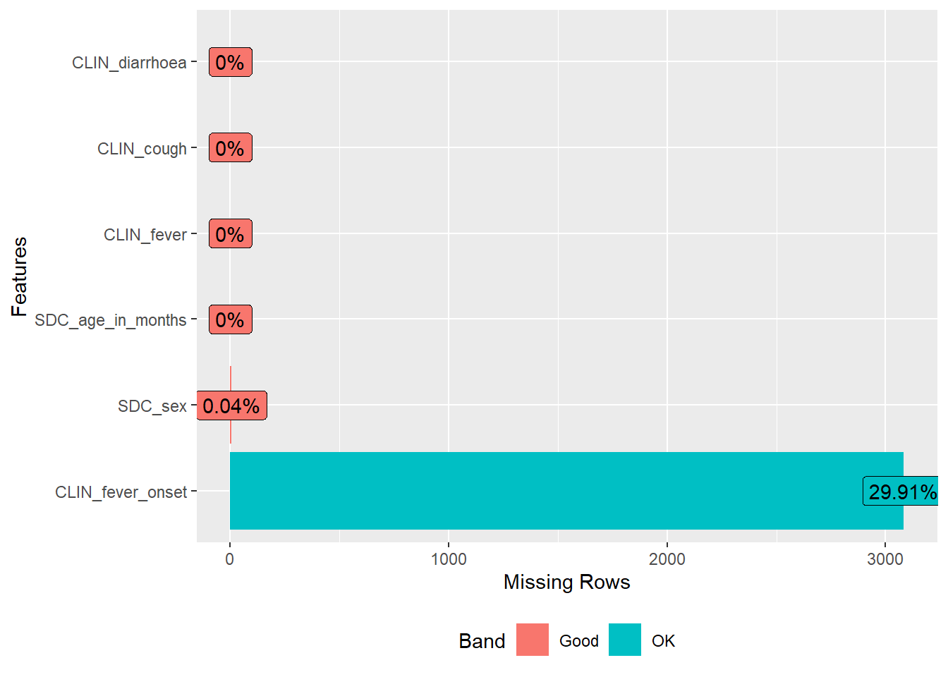
DataExplorer::plot_missing(df1)
5.11 Manipulate Python and R data
- Import dataset1.xlsx using Stata and store it in
df1
```{r}
# Write your code here
```- Import dataset1.csv using Python and store it in
df2
```{python}
# Write your code here
```- Compare
df1anddf2. Can you indicate what variable has been modified in dataset1 between df1 and df2?
Tip
Use the R function comparedf
```{r}
# Write your code here
```- Import dataset1.xlsx using Stata and store it in
df1
```{r}
library(RStata)
df1 <- RStata::stata("import excel ./data/dataset1a.xlsx",
                     data.out = TRUE)
```
. import excel ./data/dataset1a.xlsx
(7 vars, 10,309 obs)- Import dataset1.csv using Python and store it in
df2
```{python}
import pandas as pd
df2 = pd.read_csv('./data/dataset1b.csv')
```- Compare
df1anddf2.
```{r}
library(reticulate)
arsenal::comparedf(df1, py$df2)
```
Compare Object
Function Call:
arsenal::comparedf(x = df1, y = py$df2)
Shared: 0 non-by variables and 10308 observations.
Not shared: 14 variables and 1 observations.
Differences found in 0/0 variables compared.
0 variables compared have non-identical attributes.